Back home

7 November 2018

NYC subway data with Kafka Streams and JHipster (part 2 of 2)

tags: Apache Kafka - JHipster

In part 1 of this blog post I explained how to retrieve data from the MTA feed and publish it to Kafka. I will now explain how to easily visualize this data using InfluxDB and Grafana. InfluxDB is an open-source time series database that can be used as a data source for Grafana. Grafana is an open-source, general purpose dashboard and graph composer, which runs as a web application. Grafana will be used to visualize the number of active subways for each line through a day and see how this number changes with time.

All the code of this blog post can be found on this GitHub repository and I recommend cloning it instead of copying the code examples.

Saving measurements to InfluxDB

InfluxDB setup with the microservice

Starting an InfluxDB instance can be achieved using the below Docker command:

docker run -p 8086:8086 -v $PWD:/var/lib/influxdb influxdb

A database is required to save the measurements, here is the cURL command to create a database named mta:

curl -G http://localhost:8086/query --data-urlencode "q=CREATE DATABASE mta"

The microservice can now connect to the instance and start saving measurements in the mta database using the Java driver. In order to use the Java driver, the below Maven dependency must be added first:

<dependency>
    <groupId>org.influxdb</groupId>
    <artifactId>influxdb-java</artifactId>
    <version>2.14</version>
</dependency>

Configuring the java client is very simple and the InfluxDB interface will later be used to query the database.

// Init influxDB
InfluxDB influxDB = InfluxDBFactory.connect("http://127.0.0.1:8086", "root", "root");
influxDB.setDatabase("mta");

Measurements saving

In part 1, the Kafka mta-stream topic was used to store the results from the streaming process. This topic will be used to save each message in InfluxDB since a message represents the number of active subways for a given line and time.

@StreamListener(MessagingConfiguration.MtaStream.INPUT)
public void saveSubwayCount(SubwayCount subwayCount) {
    // Save measurement in influxdb
    influxDB.write(Point.measurement("line")
        .time(subwayCount.getStart().toEpochMilli(), TimeUnit.MILLISECONDS)
        .tag("route", subwayCount.getRoute())
        .addField("count", subwayCount.getCount())
        .build());
}

The method above gets triggered when a message is published in the mta-stream topic and will then write the message in InfluxDB. Spring Cloud Stream makes things simple by converting the Kafka message from a JSON format to the custom SubwayCount class.

InfluxDB’s measurement is conceptually similar to a table and all messages are inserted in the line measurement. The subway’s route is used as a tag to allow filtering when it will be used in Grafana. There is only one field for the point and it is the number of active subways. Finally the time of the point is the start timestamp of Kafka’s window.

Grafana configuration and dashboard creation

Once again, thanks to Docker for making the Grafana setup easy:

docker run -d -p 3000:3000 grafana/grafana

A data source for InfluxDB must be created in order to build a dashboard, here is a screenshot of my configuration:

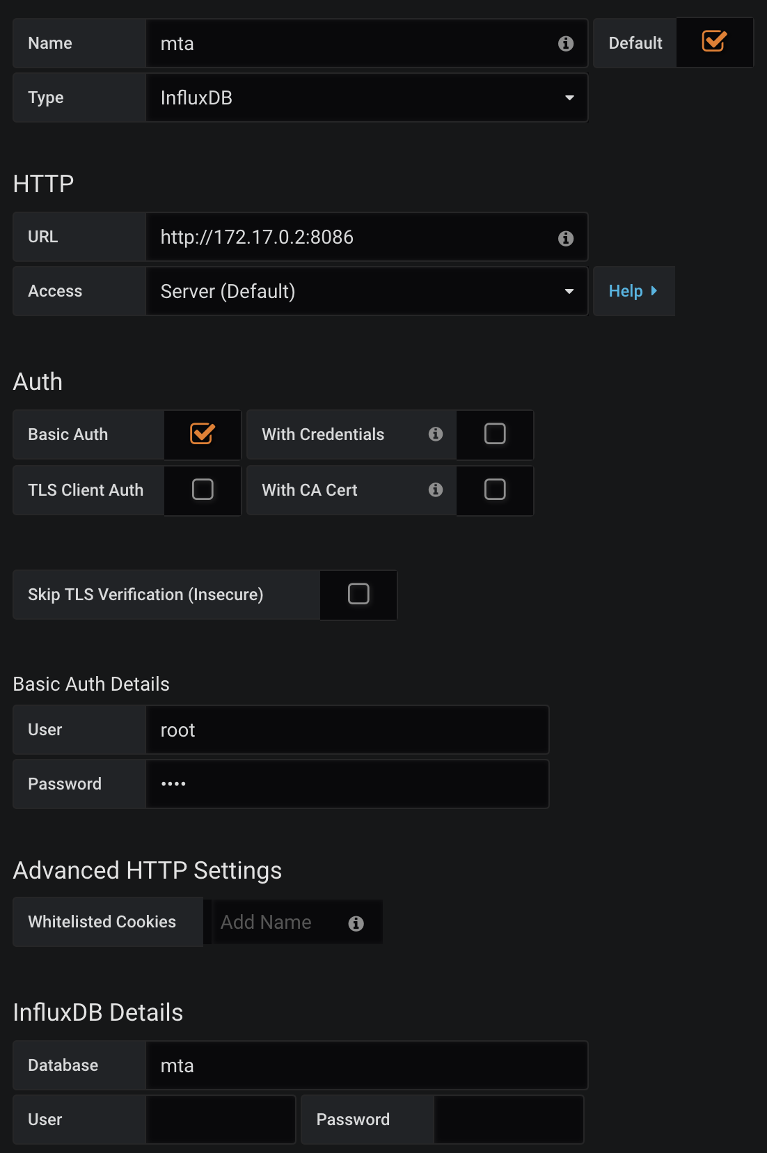
The IP must be the one of the InfluxDB’s container, it can be retrieved using the command below:

docker inspect -f '' container_name_or_id

Any dashboard can be created with the datasource. I decided to have one with a panel that will display the number of subways per line.

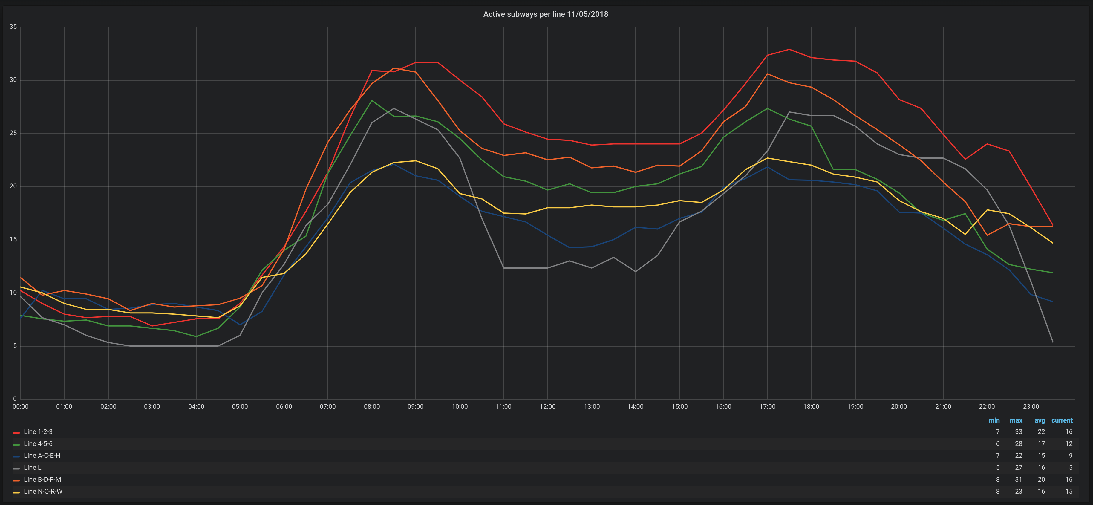
Lines are grouped to avoid having too many series and the value is the average number of running trains for a 30mins interval. The above screenshot shows the busiest lines on Monday, November 5, 2018 which is a regular work day.

This JSON configuration contains a dashboard with the panel from the screenshot and it can be easily imported in a different Grafana instance.

Conclusion

From the screenshot, we can see that the two times when the number of active subways reach its peak are 9am and 5pm. The time of the day where the number is the lowest is between midnight and 5am. The red line (or 1-2-3) is the one with the most running trains on average during a day which makes sense since it is one of the longest lines.

Using JHipster with Kafka and Spring Cloud Stream is pretty straightforward and the integration with the MTA API was easy to do. Setting up InfluxDB/Grafana with Docker takes a few minutes and it gives you a nice way to visualize the data. The next step would be to differentiate the direction for each line because there is probably a small difference between two directions of the same line.